This study was conducted in a Gobi Desert region in the middle reaches of the Heihe River Basin, Gansu Province, Northwest China (Figs. 1a and b). The study area (39° 24′ -39° 29′ N, 100° 08′ -100° 12′ E; 1390-1470 m a.s.l.), covering an area of approximately 40 km² (8 km× 5 km), is bordered by a young oasis to the southwest, a remnant of the Qilian Mountains to the north, and an extension of the Badain Jaran Desert to the southeast (Fig. 1c). The area is characterized by a temperate arid climate with the annual mean temperature of 7.6° C and the mean annual precipitation of 117 mm. It should be noted that about 65% of annual total precipitation occurred in the rainy season spanning from July to September. The mean annual pan-evaporation is 2390 mm, and the mean annual wind speed is 3.2 m/s (with the dominant windy days occurring between March and May). The zonal soil is classified as grey-brown desert soil (He and Zhao, 2004) and is derived from the fluvial-alluvial deposits (Su and Yang, 2008). Soil textures range from sand to clay. The study area has been fenced and protected from grazing for the purpose of vegetation restoration. Vegetation cover is spatially heterogeneous, with patches of shrubs and sub-shrubs interspersed within a matrix of bare soil.

Fig. 1

	Figure Option ViewDownloadNew Window
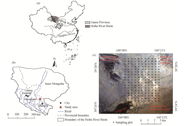	Fig. 1 Locations of the study area (a, b) and the sampling plots (c)

A quantitative vegetation survey was carried out in mid-August 2012, i.e., the vigorous growth period of plant species. We carried out the survey based on 187 regular grids (each area of 500 m× 500 m) and the positions were recorded with a portable Garmin GPS receiver (resolution of 3 m). Correspondingly, a total of 187 shrub sampling plots with a distance of ~480 m from each other were selected. The average size of each plot was 400 m² (20 m× 20 m). In each sampling plot, three herbaceous sampling quadrats with an area of 2 m× 2 m each were randomly set. All plant species were identified and recorded, and the abundance, height, and cover of each species were measured and recorded. Specifically, the abundance was determined by counting the individuals of each species; the height was measured from the soil surface to the highest point of the plant; and the cover was estimated as the percentage ratio of the crown size to the plot size for the shrub species and estimated using the visual method for the herbaceous species (Sutherland, 1999).

In each sampling plot, five soil samples were randomly collected from the upper soil layer (0-10 cm) and were mixed as one composite sample. Those soil samples (187 in total) were air dried, weighed, and sieved by a 2-mm mesh. Then, each of soil samples was divided into the coarse (particle size > 2 mm) and fine (particle size ≤ 2 mm) fractions. The coarse samples were reweighed to determine the gravel content. The fine samples were further separated into two parts. One part was used to determine the particle-size distribution with a Mastersizer 2000 particle-size analyzer (Malvern Instruments, Malvern, England). The other was passed through a 0.25-mm mesh and then used to determine soil organic carbon content using potassium dichromate/wet combustion (Nelson and Sommers, 1982). In each sampling plot, five soil samples (at the same locations with the above five samples) were also collected from the upper soil layer (0-10 cm) to determine saturated hydraulic conductivity, bulk density, and total porosity. The saturated hydraulic conductivity was measured using the constant hydraulic head method (Klute and Dirksen, 1986), and bulk density and total porosity were measured using the gravimetric method. For each plot, the five replicate measurements were averaged to reduce the influence of gravels on the measurements.

In this study, Patrick richness index (R), Shannon-Wiener diversity index (H’), Simpson’ s dominance index (D), and Pielou’ s evenness index (J) were selected to evaluate the plant species diversity (Zhang et al., 2003).

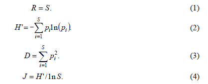
Where, S is the number of species recorded in each sampling plot, and p_i is the relative importance value of speciesi in each sampling plot. The relative importance value of species i in each sample plot was calculated as: p_i=(relative cover+relative height+relative abundance)/3 (Li et al., 2006).

Descriptive statistical analyses (including maximum, minimum, mean, median, kurtosis, skewness, standard deviation (SD), and coefficient of variation (CV)) were firstly used to identify the variation trends of plant species diversity indices. The normality of the data was tested using the one-sample Kolmogorov-Smirnov (K-S) test. It should be pointed out that the natural logarithmic transformations were applied where necessary for meeting the normality requirements of the geostatistical analyses. Furthermore, correlation analysis was used to determine the relationships between plant species diversity and environmental factors.

Estimating the variability of plant species diversity indices at different spatial scales is important for effectively sampling vegetation in the field and accurately predicting the changes in plant species diversity. In this study, we re-sampled the subsets of plot allocations of different sizes for all sampling plots (n=187) to detect the variability of plant species diversity indices associated with the size of the re-sampling area. We assigned integral multiples of 1 km to the east-west and north-south directions within the study area to generate two sets of options. Specifically, 5 re-sampling options were generated along the east-west direction and 8 re-sampling options were generated along the north-south direction. The random combination of these two sets of options thus yielded 40 potential re-sampling options (corresponding to 40 re-sampling areas). It should be noted that different re-sampling options may obtain the same re-sampling area, e.g., 1 km× 4 km and 2 km× 2 km were the same within the study area and thus they should be excluded. Totally, 24 re-sampling areas were obtained (see Zhang and Shao (2015)). The variability of plant species diversity indices in an area was calculated by averaging the coefficients of variation (CVs) of all possible re-sampling options with the same area.

Semivariograms were used to quantify the spatial dependence of plant species diversity indices and to provide the input parameters of ordinary kriging interpolation. The semivariogram can be calculated as follows (Yost et al., 1982):

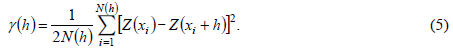
Where, Z(x_i) and Z(x_i+h) are observation values at positions x_i and x_i+h, respectively; and N(h) is the number of pairs of sample points separated by the lag distance h.

The experimental variogram was calculated for several lag distances and then were fitted with theoretical models, such as spherical, exponential, Gaussian, and linear models. Then, the best-fitted semivariogram model with the smallest residual sum of squares (RSS) and the highest coefficient of determination (R²) was selected. The model provided the input parameters for the ordinary Kriging interpolation to predict the spatial pattern of plant species diversity. The parameters included: (1) nugget (C₀); (2) sill (C+C₀); (3) nugget ratio (C₀/(C+C₀)); and (4) range (A) (Schneider et al., 2011). The nugget (C₀) represents the undetectable measurement error, inherent heterogeneity, or the fine-scale variability. The sill (C+C₀) is the upper limit of the semivariogram model, representing the total variation. The nugget ratio (C₀/(C+C₀)) can be used as a criterion for classifying the spatial autocorrelations among variables, with ratios of < 0.25, 0.25-0.75, and > 0.75 representing strong, moderate, and weak spatial autocorrelations, respectively (Cambardella et al., 1994). The range (A) of spatial dependency is the separation distance at which the sill is reached. Samples separated by distances shorter than the range (A) are spatially related, whereas samples separated by distances longer than the range (A) are not spatially related.

The geostatistical analysis was performed with GS+ version 7.0 (Gamma Design Software, Plainwell, USA), and the contour maps of ordinary Kriging interpolation were produced with the GIS program ArcView version 3.3 and its extension module Spatial Analysis version 2.0 (ESRI Inc., Redlands, USA).

Plant species composition in the study area was simple, mainly with xerophytic or super-xerophytic shrubs, sub-shrubs, and annual and perennial herbaceous plants (Table 1). A total of 42 species belonging to 16 families and 39 genera were recorded in the 187 plots. The frequency of occurrence was low for most species, with the value < 10.0% for 23 species. At the family level, Compositae, Chenopodiaceae, Zygophyllaceae, Leguminosae, and Gramineae were the most abundant families, totally accounting for 61.9% of the total recorded species. At the species level, herbaceous species (including annual and perennial herbaceous plants) occupied a large proportion of the total recorded species (71%). The most frequent herbaceous species were Halogeton arachnoideus, Artemisia sphaerocephala, Allium mongolicum, Salsola ruthenica, and Zygophyllum fabago, with a frequency of occurrence > 60% for each. However, at the community level, shrub species (including shrubs and sub-shrubs) represented the major part of the plant communities, covering 90% of the land surface. The dominant shrub species wereReaumuria songarica and Nitraria sphaerocarpa, with a frequency of occurrence > 90% for each.

Table 1

Table 1

Table 1 Characteristics of the recorded plant species in the sampling plots Species name Family Life form Frequency (%) Species name Family Life form Frequency (%) Nitraria sphaerocarpa Zygophyllaceae Sh 99 Chloris virgata Poaceae Ah 33 Ephedra przewalskii Ephedraceae Sh 6 Tribulus terrestris Zygophyllaceae Ah 2 Caragana brachypoda Leguminosae Sh 2 Chenopodium glaucum Chenopodiaceae Ah 1 Atraphaxis frutescens Polygonaceae Sh 1 Allium mongolicum Liliaceae Ph 66 Tamarix ramosissima Tamaricaceae Sh 1 Swainsonia salsula Leguminosae Ph 19 Calligonum mongolicum Polygonaceae Sh 3 Scorzonera divaricata Compositae Ph 3 Reaumuria songarica Tamaricaceae Ss 94 Zygophyllum fabago Zygophyllaceae Ph 63 Kalidium gracile Amaranthaceae Ss 38 Arnebia szechenyi Boraginaceae Ph 28 Zygophyllum xanthoxylon Zygophyllaceae Ss 1 Astragalus discolor Leguminosae Ph 12 Asterothamnus centrali-asiaticus Compositae Ss 12 Artemisia sphaerocephala Compositae Ph 70 Hedysarum scoparum Leguminosae Ss 2 Artemisia scoparia Compositae Ph 17 Sympegma regelii Chenopodiaceae Ss 8 Artemisia frigida Compositae Ph 27 Bassia dasyphylla Chenopodiaceae Ah 26 Peganum harmala Zygophyllaceae Ph 2 Halogeton arachnoideus Chenopodiaceae Ah 93 Stipa gobica Poaceae Ph 34 Salsola ruthenica Amaranthaceae Ah 65 Cynomorium songaricum Cynomoriaceae Ph 1 Suaeda microphylla Chenopodiaceae Ah 2 Limonium aureum Plumbaginaceae Ph 9 Agriophyllum squarrosum Chenopodiaceae Ah 2 Cynanchum chinense Asclepiadaceae Ph 1 Echinops gmelini Compositae Ah 14 Peganum multisectum Zygophyllaceae Ph 1 Lappula patula Boraginaceae Ah 1 Allium polyrhizum Alliaceae Ph 1 Neopallasia pectinata Compositae Ah 1 Cistanche deserticola Orobanchaceae Ph 1 Eragrostis pilosa Poaceae Ah 19 Achnatherum splendens Poaceae Ph 1 Note: Sh, shrub; Ss, sub-shrub; Ah, annual herbaceous; Ph, perennial herbaceous.

Table 1 Characteristics of the recorded plant species in the sampling plots

The statistical parameters of the four plant species diversity indices (i.e., Patrick richness index (R), Shannon-Wiener diversity index (H’), Simpson’ s dominance index (D), and Pielou’ s evenness index (J)) are shown in Table 2. It can be seen that the ranges of R, H’, D, and Jwere 2.00-21.00, 0.50-1.90, 0.18-0.76, and 0.24-0.94, respectively. All of those four indices were moderately spatially variable, with the values of CVs (coefficients of variation) ranging between 21.6% and 40.7%. The coefficients of skewness and kurtosis together with the non-parametric K-S tests showed that the statistical distributions of R and D were positively skewed (P< 0.05) and that the statistical distributions of H’ and R were normally distributed (P> 0.05). The log-transformed data of both H’and R, however, passed the K-S tests at the 0.05 significance level and then consequently could be used for the geostatistical analyses.

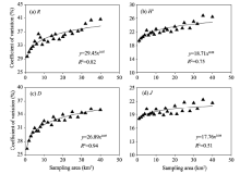
The CVs of all plant species diversity indices increased with increasing sampling area (Fig. 2). The variations of CVs for R and D with increasing sampling area could be best fitted with power functions, with R² values of 0.82 and 0.94, respectively (P< 0.05). The variations of CVs for H’ and J with increasing sampling area were best fitted with linear functions, with R² values of 0.84 and 0.60, respectively (P< 0.05). But it should be added that they were also well fitted with power functions, with R² values of 0.75 and 0.51, respectively (P< 0.05). It seems that the power functions may be more theoretically reasonable because the CVs should be zero when the sampling area is zero.

Table 2

Table 2

Table 2 Descriptive statistics of plant species diversity indices Statistical parameter Diversity index R H’ D J Maximum 21.00 1.90 0.76 0.94 Minimum 2.00 0.50 0.18 0.24 Mean 9.05 1.25 0.37 0.60 SD 3.68 0.33 0.13 0.13 CV 40.70 26.25 35.40 21.66 Skewness 0.37 -0.18 0.86 -0.08 Kurtosis -0.31 -0.51 0.06 -0.31 P of K-S test 0.044 0.098 0.003 0.375 Note: SD, standard deviation; CV, coefficient of variation; R, Patrick richness index; H’, Shannon-Wiener diversity index; D, Simpson’ s dominance index; J, Pielou’ s evenness index.n=187.

Table 2 Descriptive statistics of plant species diversity indices

Fig. 2

	Figure Option ViewDownloadNew Window
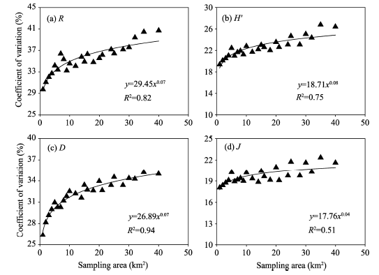	Fig. 2 Relationships of coefficients of variation for the four plant species diversity indices with sampling areas. (a), Patrick richness index (R); (b), Shannon-Wiener diversity index (H’); (c), Simpson’ s dominance index (D); (d), Pielou’ s evenness index (J).

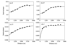
The semivariograms for R and H’ were optimally fitted by Gaussian models, whereas the semivariograms for D and J were best fitted by exponential models (Table 3; Fig. 3). All of the models were satisfactory (with R² values varying from 0.82 to 1.00), suggesting that these models can well represent the spatial patterns of plant species diversity indices in the study area.

Table 3

Table 3

Table 3 Parameters of the semivariogram models estimated for the four plant species diversity indices Diversity index Model Nugget (C0) Sill (C+C0) Nugget ratio (C0/(C+C0)) Range (A; m) R2 R Gaussian 7.190 14.410 0.499 3681 0.99 H’ Gaussian 0.049 0.115 0.422 2969 1.00 D Exponential 0.007 0.022 0.312 7890 0.99 J Exponential 0.002 0.017 0.108 1218 0.82 Note: R2, coefficient of determination; R, Patrick richness index; H’, Shannon-Wiener diversity index; D, Simpson’ s dominance index; J, Pielou’ s evenness index.

Table 3 Parameters of the semivariogram models estimated for the four plant species diversity indices

Fig. 3

	Figure Option ViewDownloadNew Window
	Fig. 3 Semivariograms for the four plant species diversity indices. (a), R; (b), H’; (c), D; (d), J.

Both nugget (C₀) and sill (C+C₀) were higher for R than for other three indices (H’, D, andJ), which may be attributable to the high value of R itself (Table 3). The nugget (C₀) and sill (C+C₀) for other three indices (H’, D, and J) varied in the order of H’> D> J (Table 3), indicating a higher degree of spatial variability for H’ than for D and J. The nugget ratios (C₀/(C+C₀)) for the four indices indicated moderate spatial autocorrelations for R, H’, and D (ratios of 0.31-0.50) and a strong spatial autocorrelation for J(ratio of 0.11). Furthermore, the spatial autocorrelations (i.e., D, 7890 m; R, 3681 m; H’, 2969 m; and J, 1218 m) indicated that the degree of spatial dependence for the four plant species diversity indices was in the order of D> R> H’> J.

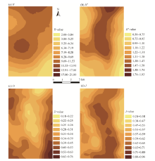
The spatial patterns of R and H’ were highly dependent on the location within the study area. Generally speaking, R and H’ increased gradually from southwest (near the oasis) to north (surrounded by low mountains) and decreased gradually towards the southeastern region that joins with the Badain Jaran Desert (Figs. 4a and b). The spatial pattern of D, however, displayed an opposite trend to those of R and H’, with high D values distributed in the areas near the oasis and desert (Fig. 4c). Being different from the above three indices, J exhibited an irregular spatial pattern (Fig. 4d). As shown in Figure 4d, the plant species were more evenly distributed in the central area.

Fig. 4

	Figure Option ViewDownloadNew Window
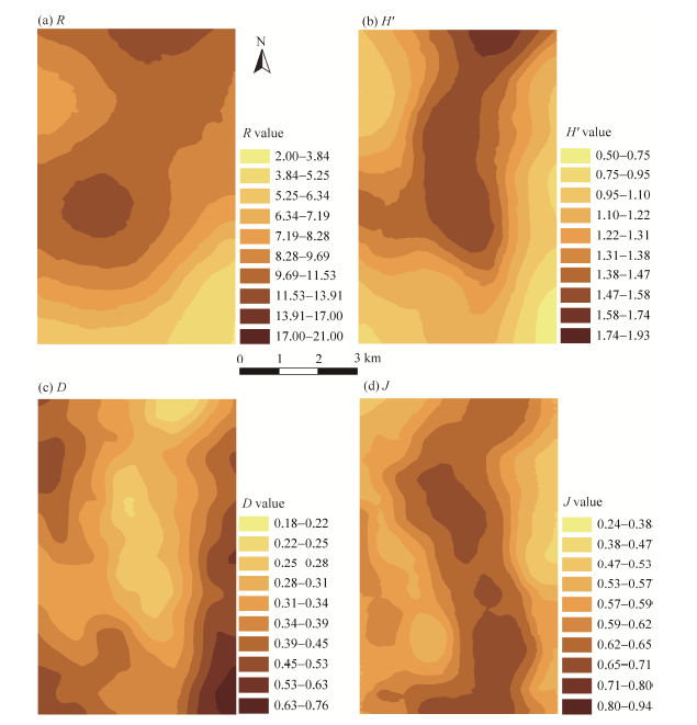	Fig. 4 Spatial patterns of the four plant species diversity indices across the study area. (a), R; (b), H’; (c), D; (d), J.

The correlation coefficients for the relationships between plant species diversity indices and environmental factors (including elevation and soil properties) are presented in Table 4, and the correlation coefficients for the relationship between the environmental factors are presented in Table 5. As shown in Table 4, J was not significantly correlated with any of the factors considered (P> 0.05), indicating that the differences in the spatial distribution of plant species were not affected by these factors. However, R, H’, and D were significantly correlated with elevation and all soil properties considered (P< 0.05) with an exception of soil organic carbon content (P> 0.05), implying that elevation and soil properties (with an exception of soil organic carbon content) play important roles in the spatial variability of plant species diversity. Specifically, R and H’ were significantly and negatively correlated with silt content (P< 0.01), clay content (P< 0.01) and total porosity (P< 0.01), and were positively correlated with elevation (P< 0.01), bulk density (P< 0.01), gravel content (P< 0.01), sand content (P< 0.01), and saturated hydraulic conductivity (P< 0.05). Furthermore, the correlations between D and environmental factors were opposite to those for R and H’ (Table 4).

Table 4

Table 4

Table 4 Pearson’ s correlation coefficients between plant species diversity indices and environmental factors Environmental factor R H’ D J Elevation 0.40* * 0.29* * -0.26* * -0.07 BD 0.37* * 0.29* * -0.24* * -0.05 Gravel 0.46* * 0.32* * -0.25* * -0.04 Sand 0.37* * 0.27* * -0.20* * -0.08 Silt -0.36* * -0.26* * 0.20* * 0.08 Clay -0.37* * -0.27* * 0.20* * 0.08 SOC -0.11 -0.05 0.00 0.06 Ks 0.18* 0.18 * -0.14* 0.08 TPo -0.38* * -0.32* * 0.29* * 0.04 Note: BD, bulk density; SOC, soil organic carbon; Ks, saturated hydraulic conductivity; TPo, total porosity. * and * * indicate that the correlation is statistically significant at P< 0.05 and P< 0.01 levels, respectively.

Table 4 Pearson’ s correlation coefficients between plant species diversity indices and environmental factors

Table 5

Table 5

Table 5 Pearson’ s correlation coefficients among the environmental factors BD Gravel Sand Silt Clay SOC Ks TPo Elevation 0.38* * 0.39* * 0.47* * -0.47* * -0.46* * -0.27* * -0.12 -0.41* * BD 1.00 0.41* * 0.66* * -0.67* * -0.63* * -0.41* * 0.15* -0.95* * Gravel 1.00 0.45* * -0.46* * -0.43* * -0.20* * 0.14* -0.42* * Sand 1.00 -0.98* * -0.99* * -0.68* * 0.18* -0.70* * Silt 1.00 0.95* * 0.68* * -0.17* 0.73* * Clay 1.00 0.66* * -0.18* 0.66* * SOC 1.00 -0.16* 0.43* * Ks 1.00 -0.16* TPo 1.00 Note: * and * * indicate that the correlation is statistically significant at P< 0.05 and P< 0.01 levels, respectively.

Table 5 Pearson’ s correlation coefficients among the environmental factors

The shrub species (including shrubs and sub-shrubs) and herbaceous species (including annual and perennial herbaceous plants) in the study area were mainly xerophytes or super-xerophytes. Shrub species generally represented the major part of the plant communities, covering 90% of the land surface. In contrast, herbaceous species only occurred individually in rather localized spots. However, these herbaceous species occupied a large proportion of the total recorded species (71%) and thus played important roles in the structure of the plant communities and in the functions of the ecosystems in the study area.

It was previously reported that plant species diversity is high in favorable environments and low in harsh environments (Danin, 1976). Our study area (i.e., a Gobi Desert region) is dominated by a dry climate with low precipitation, high evaporation, and severe wind erosion. These environmental conditions are more suitable for the survival of deep-rooted shrub species (e.g, R. songarica and N. sphaerocarpa) that have high resistance to drought and sand burial. In contrast, some other shrub and herbaceous species (such as Ephedra przewalskii, Tamarix ramosissima, Peganum multisectum, Lappula patula) can only live in occasionally favorable environmental conditions and can be considered as opportunists. This region had a low species evenness and diversity, precisely because of the higher number of opportunists present and lower number of individuals (Ricotta and Avena, 2003). H’ in our study area (range of 0.50-1.90) was low and it was generally within the H’ ranges reported in the other desert regions in China, e.g., the oasis-desert ecotone in Fukang of Xinjiang (0.48-1.57; Zhang et al., 2003), the northeastern Ulan Buh Desert in Inner Mongolia (0.60-2.98; Wang et al., 1996), and the southeastern Tengger Desert in Inner Mongolia (0.60-1.63; Kong and Shen, 2003). Those results indicated that plant species diversity of desert plant communities is universally low.

In this study, all the four plant species diversity indices (i.e., R, H’, D, and J) were spatially varying, which can be attributed to the heterogeneity of the environmental factors. Different plant species have different resource niches and can be competitively dominant in different environments (Gundale et al., 2011). The variations in environmental factors will thus result in the spatial variability of species distribution and diversity (Reynolds et al., 2007). Our results demonstrated that plant species diversity was not distributed randomly in space. Instead, they followed distinctive spatial patterns, being rather consistent with the findings of the latest studies (Irl et al., 2015; Fibich et al., 2016). R, H’, and D exhibited moderate spatial autocorrelations, indicating that the spatial variability of these three indices was regulated by both intrinsic factors (i.e., soil-forming processes) and extrinsic factors (i.e., desert management and human activities). Being different from those three indices above mentioned, J showed a strong spatial autocorrelation, which can be attributed to the intrinsic factors (i.e., soil-forming processes).

Our results also showed that the variability of plant species diversity was spatially scale-dependent and was increased with increasing sampling area (size). It was widely reported that environmental factors could influence the distribution of plant species at different spatial scales (e.g., Muñ oz-Reinoso and Novo, 2005; Chandy and Gibson, 2009). At large spatial scales, parental material, climate, and geological history are usually the major factors; while at small spatial scales, ecological interaction among the plant species may be the dominant factor. Furthermore, the environmental factors operating at small spatial scales may greatly influence the distribution of plant species at large spatial scales (Zuo et al., 2012). With increasing sampling area, the driving factors of the variability of plant species diversity above mentioned may become increasingly complex and heterogeneous, thus resulting in higher spatial variability of plant species diversity. In this study, the positive power-function relationship between the CVs of plant species diversity indices and the sampling area indicated that the spatial pattern of plant species diversity was strongly scale-dependent at small spatial scales. This may be due to the discontinuous, patchy, and mosaic distributional patterns of plant species. At small spatial scales, competitive and inter-dependent relationships between plant species are strong in the Gobi Desert region, and many species cluster together to avoid the interference of shifting sand. In contrast, at large spatial scales, due to the flat terrain in the Gobi Desert region, the topographic and hydrogeomorphic conditions are more consistent, thus sampling area (size) is less important in controlling the plant species diversity (He et al., 2006). In our study, an area of 10 km² seems to be the turning point, below which the influence of the changes in sampling area on the plant species diversity was much more obvious (see Fig. 2). This finding indicated that an area of 10 km² is an optimal option to represent the plant species diversity and it could be used as a reference size for determining the sampling area in the field investigation in dry desert regions.

Variations of plant species diversity are linked with many environmental factors, such as climate, soil, and topography (Huerta-Martí nez et al., 2004; Zuo et al., 2012). Due to the small size of the study area, climatic factors were disregarded in this study. The topographical features and soil properties were thus most likely responsible for the spatial pattern of plant species diversity.

Elevation is an important topographical property influencing the spatial pattern of plant species diversity. R and H’ in our study were significantly and positively correlated with elevations, suggesting that species composition was variable at higher elevations. Previous studies reported that elevation can indirectly regulate the distribution of plant species by influencing the redistribution of soil properties, such as soil moisture, soil nutrients (accumulation and transportation), and soil particle composition (Fu et al., 2004; Zuo et al., 2008). The positive relationship of elevation with R and H’ may be a consequence of the combined contributions of soil properties (Table 5). In fact, the regions at higher elevations in this study were mainly in the transitional zone between the mountains and the Gobi Desert. The micro-topography (such as the runoff gullies) and various soil substrates fragmented the habitats, thus promoting the coexistence of more plant species and increasing the diversity of plant species. In contrast, other previous studies have reported a hump-shaped pattern between species diversity with elevation (Vá zquez Garcí a and Givnish, 1998; Wang et al., 2003). This discrepancy may be due to the elevation range sampled in the field. The elevation gradients were actually rather small in our study. Moreover, Lomolino (2001) demonstrated that the pattern of diversity-elevation gradients might depend largely on the patterns of co-variation and interaction among the geographically explicit variables.

Soil properties are decisive factors determining the distribution of plant species in arid and semi-arid areas (Maestre et al., 2003). Soil texture and bulk density, the most fundamental physical properties, determine the pore size and shape, and thereby control the exchange and uptake of water, nutrients, and oxygen, thus influencing the growth and distribution of plant species (Arekhi et al., 2010). Gravels in the surface and subsurface soil layers generally modulate water infiltration and evapotranspiration, normally increasing the water availability for plant uses (Unger, 1971). As expected, the spatial distribution of plant species diversity in the study area was highly correlated with the aforementioned soil physical properties. As soil silt and clay contents increased and gravel content decreased, soil bulk density and saturated hydraulic conductivity decreased and total porosity increased, resulting in an increase in the moisture-holding capacity of the soil. Generally speaking, wetter habitats always have a higher vegetation cover and biomass (Li et al., 2004), which in turn could increase the intensity of species competition and may allow a few species with strong competitive abilities to dominate, thus decreasing the species diversity (Abrams, 1995; Mittelbach et al., 2001). In contrast, the growth of plant species in drier habitats is restricted by coarse-textured soil with lower soil moisture, and species can thus coexist in close proximity without directly competing for resources (Abrams, 1995).

The shelter belts in the study region near the oasis functioned as natural barriers to reduce wind velocity and intercept the fine materials, providing a wetter habitat for a few species, e.g., N. sphaerocarpa, R. songarica, Kalidium gracile, and H. arachnoideus, which impeded the survival and development of plant species with less competition vigor in this relatively wet habitat. Plant species with less competition vigor were stunted and gradually lost their competitive advantages towards the northern direction (coarse-textured soils with higher contents of gravel and coarse sand). The most representative plant species were K. gracile and H. arachnoideus and their dominance was resulted from the relatively high soil moisture. Those plant species with less vigor, (e.g., K. gracile, H. arachnoideus, Ephedra przewalskii, Asterothamnus centrali-asiaticus, Allium mongolicum, and Stipa gobica) were thus able to colonize in the northern part, so that the dominant species were not apparent and competitive exclusion did not occur.

In our study, plant species diversity indices were unexpectedly not significantly correlated with soil organic carbon. Other studies, however, have suggested that the distribution of plant species diversity was strongly influenced by soil organic carbon (Yang et al., 2009; Chigani et al., 2012). As reported by Grime (1979), species diversity will be highest at intermediate levels of soil fertility and will be constrained at low levels of soil fertility. Furthermore, high levels of soil fertility may lead to competitive exclusion. Plant growth in this harsh Gobi Desert region (i.e., the study area) may be constrained by many factors, such as the amounts of soil water content and salt content and the availability of soil nutrients (e.g., total nitrogen, and available potassium). The effect of soil organic carbon on species diversity may have been overshadowed by other factors.