SHA Zongyao, XIE Yichun, TAN Xicheng, BAI Yongfei, LI Jonathan, LIU Xuefeng. , Assessing the impacts of human activities and climate variations on grassland productivity by partial least squares structural equation modeling (PLS-SEM). Journal of Arid Land, 2017, 9(4): 473-488.
Assessing the impacts of human activities and climate variations on grassland productivity by partial least squares structural equation modeling (PLS-SEM)
SHA Zongyao1,*, XIE Yichun2, TAN Xicheng1, BAI Yongfei3, LI Jonathan4, LIU Xuefeng5
1 International Software School, Wuhan University, Wuhan 430079, China
2Department of Geography and Geology, Eastern Michigan University, Ypsilanti, MI 48197, USA
3Institute of Botany, Chinese Academy of Sciences, Beijing 100093, China
4Department of Geography & Environmental Management, University of Waterloo, 200 University Avenue West, Waterloo,Ontario N2L 3G1, Canada
5 School of Communication and Information Engineering, Shanghai University, Shanghai 200072, China
The cause-effect associations between geographical phenomena are an important focus in ecological research. Recent studies in structural equation modeling (SEM) demonstrated the potential for analyzing such associations. We applied the variance-based partial least squares SEM (PLS-SEM) and geographically-weighted regression (GWR) modeling to assess the human-climate impact on grassland productivity represented by above-ground biomass (AGB). The human and climate factors and their interaction were taken to explain the AGB variance by a PLS-SEM developed for the grassland ecosystem in Inner Mongolia, China. Results indicated that 65.5% of the AGB variance could be explained by the human and climate factors and their interaction. The case study showed that the human and climate factors imposed a significant and negative impact on the AGB and that their interaction alleviated to some extent the threat from the intensified human-climate pressure. The alleviation may be attributable to vegetation adaptation to high human-climate stresses, to human adaptation to climate conditions or/and to recent vegetation restoration programs in the highly degraded areas. Furthermore, the AGB response to the human and climate factors modeled by GWR exhibited significant spatial variations. This study demonstrated that the combination of PLS-SEM and GWR model is feasible to investigate the cause-effect relation in socio-ecological systems.
Natural grasslands and savannas occupy nearly half of the terrestrial area of the globe (Moore, 1966; Chapin et al., 2001) and provide important services to human societies. Grassland vegetation not only provides food for livestock but also contributes considerably to the global carbon recycle. Grasslands are sensitive to human activities and weather variations (Lauenroth et al., 1999; Gang et al., 2014). Climate change and human interference are commonly recognized as the two broad underlying drivers that lead to grassland degradation (Gang et al., 2014; Zhang et al., 2016). Understanding the factors affecting grassland productivity is increasingly critical to the conservation and, in some cases, to the restoration of these fragile ecosystems (De Luis et al., 2006; Cutler et al., 2008). The grassland ecosystem is essentially a paired socio-ecological system (SES) that involves complicated interactions related to both socio-economic activities and natural factors. Plenty of studies trying to examine the impact of human activities or climate changes on vegetation growth have been reported (e.g., Li et al., 2013). There are three levels of models in studying SES, namely, loose coupling, tight coupling, and integrated modeling (Antle et al., 2001). While much attention has been paid to studying systemic changes of ecological and economic systems independently, the attempt for taking a coupled SES approach is still rare (Stannard and Aspinall, 2011; Filatova et al., 2013; Polhill et al., 2016). Two strategies, i.e., bottom-up and top-down, are usually taken in the integrated SES modeling. The bottom-up strategy starts from decomposed elements/components and models their relationships based on some selected conceptual frameworks. On the contrary, the top-down modeling starts from the overall performance of a socio-ecological system and attributes the performance to individual elements and/or to their interaction. A systematic study frame for better discovering casual relationship in SES is still required.
Over the last decade, structural equation modeling (SEM) has been applied in many scientific disciplines (Astrachan et al., 2014; Sarstedt et al., 2014; Surridge et al., 2014). As a second-generation multivariate statistical approach, SEM has played a prominent role in the SES (Liu et al., 2014; Lowry and Gaskin, 2014). SEM possesses substantial advantages over the first generation techniques (Chin, 1998; Banerjee and Hine, 2016). SEM model, which is usually composed of a measurement model and a structural model, can reveal causal relationships through introducing latent variables that relate observable variables (indicators). The latent variables, as opposed to the observable variables, are not directly observable but inferred from the observed ones. In the measurement model (or outer model), a set of latent variables are aggregated from the observable data to form an underlying concept, which greatly reduces the dimensionality of the original variables and makes the data easier to understand (Haenlein and Kaplan, 2004; Hair et al., 2014). In the structural model (or inner model), the latent variables are connected with each other according to a substantive theory in the form of simple connected digraphs (Monecke and Leisch, 2012). The latent variables in the SEM model are divided into two classes, exogenous (without any predecessors) and endogenous (having at least a predecessor). Designed for working with multiple equations simultaneously, SEM offers a number of advantages over the traditional statistics such as regression analysis or factor analysis (Sarstedt et al., 2014). SEM has been popular in many disciplines and allows great flexibility on equation specification (Hair et al., 2009; Monecke and Leisch, 2012). Overall, SEM model provides an effective tool to assess latent variables at the measurement model and test the relationships between the latent variables on the structural model (Bollen, 1989; Hair et al., 2012).
Two most popular types of SEM modeling were identified, i.e., the covariance-based technique or CB-SEM (Jö reskog, 1993) and the variance-based partial least square or PLS-SEM (Wold, 1982, 1985). Although both modeling types share the same roots (Jö reskog and Wold, 1982), earlier studies have focused primarily on CB-SEM. In recent years, PLS-SEM has expanded rapidly with recognition of being a distinctive and innovative multivariate analysis method (Henseler et al., 2009). PLS-SEM is a soft-modeling-technique with minimum demands regarding the measurement scales, sample sizes, and residual distributions (Tenenhaus et al., 2005). It is capable of fully revealing the inner characteristics of the observed data (Bagozzi and Yi, 2012). While CB-SEM estimates model parameters so that the discrepancy between the estimated and the sample covariance matrices is minimized, PLS-SEM maximizes the explained variance of the endogenous latent variables by estimating partial model relationships in an iterative sequence of ordinary least squares (OLS) regressions (Astrachan et al., 2014). PLS-SEM is essentially a regression-based modeling approach, which uses a component-based technique in analyzing path models (Hair et al., 2012). In addition, Bayesian SEM (or simply BSEM) and hierarchical SEM (HSEM) have also been proposed to empower multiple variance analysis over the last few years. BSEM has received escalating attention in SEM applications due to its flexibility in use; HSEM, also known as multilevel SEM, analyzes hierarchically clustered data by specifying the direct and indirect causal effect between clusters (Eisenhauer et al., 2015; Fan et al., 2016). Further reading on the definitions and applications of the SEMs can be found in the literatures (e.g., Chin, 2010; Hair et al., 2011; Astrachan et al., 2014). Detailed descriptions of the development and use of PLS-SEM models are given by Hair et al. (2011, 2014) and Henseler et al. (2016).
In this paper, a PLS-SEM model was developed to assess the influence from human and climate stresses on grassland vegetation productivity in Inner Mongolia, China. As the local economy depends heavily on livestock industry (through forage supply), it is thus necessary to understand the associations between the vegetation productivity and the influencing factors. Instead of using CB-SEM, the selection of PLS-SEM is based on the following considerations. First, unlike CB-SEM that requires the multivariate normal distribution for the input data, PLS-SEM relaxes the assumption of normal distribution and can obtain explicitly the estimated latent variable scores in the process of parameter estimation (Shen et al., 2016). For most socio-ecological systems including the grassland ecosystem examined in the study, this normality assumption cannot be guaranteed. Second, PLS-SEM has the advantage of the flexibility for the use of a single measurement construct (Hair et al., 2014). In this study, we were only interested in the vegetation productivity using above-ground biomass (AGB) as the proxy, AGB being the only indicator for the endogenous variable. Third, PLS-SEM is suitable for predictive research, which is usually not the case for CB-SEM (Surridge et al., 2014; Henseler et al., 2016). We expected that the result would be helpful in predicting forage quantity for livestock industry.
The main objectives of the study were to (1) develop a PLS-SEM model for exploring the cause-effect relationships in SESs; (2) quantitatively analyze the impact of the major human and climate factors (human-climate factors hereafter) and their interactions on the grassland productivity based on the PLS-SEM model; and (3) unravel the sensitivity and spatial variability of AGB response to the human-climate factors using geographically weighted regression (GWR) modeling.
2 Materials and methods
2.1 Study area
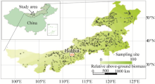
The Inner Mongolia Autonomous Region (IMAR) of China was selected as the study area (Fig. 1). As a typical grassland region of the Eurasian continent, it has an area of 1.2× 10⁶ km2, of which nearly 60% is covered with grassland vegetation. The annual average temperature in the growing season (April-September) ranges from 12.1° C in the north to 25.2° C in the south. The annual precipitation varies spatially from < 200 mm in the west to nearly 600 mm in the east, most of which is concentrated in July and August. The western section of the study area is an arid region (annual precipitation < 200 mm), the middle and the east is a semi-arid region (annual precipitation in the ranges of 200-400 and 400-600 mm, respectively) (Sha et al., 2016). Previous studies revealed that grassland productivity was affected by human activities and climate fluctuations (Mu et al., 2013; Sun et al., 2015). Specifically, the increasing human population and intensified grazing coupled with arid climate condition were identified as the primary threats to the sustainable development of the grassland ecology (Christensen et al., 2004). To the best of our knowledge, no quantitative assessment on the coupled impacts from the human activities and climate variations was conducted for the grassland system so far.
To evaluate the impact on vegetation productivity from human activities, we derived three indices, i.e., grazing intensity, road density, and urban density. A systematic field sampling of grassland was conducted in the summers of 2011-2013 and 676 samples were collected for AGB and the corresponding grazing intensities. The 676 sampling locations are shown in Figure 1. The exact sample locations were recorded using a handheld global position system (GPS) unit with an accuracy of ± 15 m. Within each sample site, five evenly distributed 1 m× 1 m quadrats were harvested for AGB. All plants in the quadrats were clipped at the ground surface and were oven-dried at 80° C for 24-48 h, or until a constant dry biomass was recorded. The grazing intensity was categorized into 6 levels, namely, extreme heavy (5), heavy (4), medium (3), moderate grazing (2), light grazing (1), and no grazing (0). Two vector layers about the road network and urbanized areas (including cities and villages) were extracted from the publicly available OpenStreetMap dataset (Zhang et al., 2015). Maps of road density and urban density were processed by the population weighted “ Point Density” and “ Line Density” analysis, respectively, and rasterized as grid layers with a spatial resolution at 1 km× 1 km to denote the accessibility to transportation and urbanized areas. The resultant pixel values indicated the influential levels from the human activities due to the accessibility to road network and urbanized areas.
To evaluate the climate impact on vegetation productivity, we regarded temperature and climate dryness as the most important indices. Annually, averaged temperature and total precipitation variables were collected from 680 meteorological stations across the entire China (http://cdc.cma.gov.cn). Those climate variables were spatially interpolated as the grid maps at 1 km× 1 km using an ANUSPLIN approach (Hutchinsom, 1999). This interpolation approach calculates and optimizes thin plate smoothing splines fitted to data sets distributed across an unlimited number of climate station locations. A general model for a thin plate spline function f(x) fitted to n data values zi at positions xi is given by,
zi=f(xi)+ε i, (1)
where, i=1, 2, ..., n, and xi represent the longitude, latitude and scaled elevation. The values of ε i are zero mean random errors and have a covariance matrix Vσ 2, where V is a known positive definite n× n matrix, usually diagonal, while σ 2 is usually unknown. The function f is estimated by minimizing:
((Z-F)TV-1Z-F)+ρ Jm(F), (2)
where, Z=(z1, …, zn)T, F=(f1, …, fn)T, and T denotes the matrix transpose, with fi=f(xi) and Jm(F) being a measure of the roughness of the spline function fdefined in terms of mth order partial derivatives of f. Digital elevation model (SRTM30 from http://srtm.usgs.gov) was resampled to the same spatial resolution as that of the climate variables and used during the interpolation process. Error analysis of the interpolated result was conducted by a comparison with the actual measurements using 53 meteorological stations located within IMAR. The climate maps were cropped to the boundary of IMAR.
From the above steps, an integrated GIS dataset was created to develop the PLS-SEM model. Climate dryness (CD_A) index was defined as the negative value of the total precipitation (i.e., precipitation), meaning that higher precipitation corresponded to lower climate dryness and vice versa. The descriptive statistics of the dataset were summarized in Table 1. As the original AGB variables were found to be highly skewed, it was square-rooted to derive a new variable AGBsqrt (square root of AGB), which was close to a normal distribution.
Fig. 1 Location of the study area and distribution of the sampling sites
Table 1
Table 1
Table 1 Parameters of partial least-square structural equation modelling (PLS-SEM) in this study
Variable
Abbr
Min
Max
Mean
SD
Skewness
Kurtosis
Above-ground biomass
AGB
5.91
938.57
152.11
126.11
2.06
6.39
Square root of AGB
AGBsqrt
2.43
30.64
11.44
4.60
0.79
0.84
Grazing intensity
Grazing
0.00
5.00
1.69
1.18
0.74
0.83
Urban density
Urban_D
0.00
6.68
1.56
1.37
1.24
0.81
Road density
Road_D
0.27
71.44
10.51
7.85
1.77
5.70
Climate dryness
CD_A
-631.44
-62.02
-369.61
83.59
-0.50
1.03
Annual average temperature
Temp_A
-2.94
9.80
3.48
2.98
-0.12
-0.85
Note: All variables except of the square root of AGB (AGBsqrt) are extracted from the corresponding layers of the GIS dataset using the coordinates of the sampling sites, n=676.
Table 1 Parameters of partial least-square structural equation modelling (PLS-SEM) in this study
2.2 PLS-SEM model specification
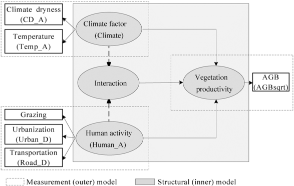
The objective of the study was to examine the effects of the human-climate factors on AGB. PLS-SEM assumes a minimum of data requirement and is an excellent tool for studying the causal relationships between multiple variables in ecological systems (Hair et al., 2009). It is worth pointing out that recent studies have suggested that climate changes and socio-economic activities could interact to create a combined or coupled effect on the grassland ecology, and thus their interactions should be taken into consideration when studying the coupled impacts of the human-climate factors for most socio-ecological systems. Accordingly, human activity (Human_A) and climate factor (Climate) along with their interaction (Interaction) were taken as the exogenous latent variables and vegetation productivity was set as the endogenous latent variable in the model specification (Fig. 2). The three variables from the previously processed dataset, including grazing intensity (Grazing hereafter), the density of urbanized area (Urban_D) and the road density (Road_D), were taken as indicators for Human_A, and the two indicators of the annual average temperature (Temp_A) and the climate dryness (CD_A) were used for Climate.
A few approaches have been proposed to analyze the interaction effect between multiple latent variables for PLS-SEM (Henseler and Chin, 2010). For instance, the product indicator approach (PIA) has been developed to quantitatively reflect the magnitude of such a coupled effect (Chin et al., 2003). In PIA, a new latent variable, or the product indicator, namely Interij, through all pairwise products of the indicators from the human-climate factors, was introduced as the interaction term,
Interij = Human_Ai× Climatej, (3)
whereiis one of the climate variables (CD_A or Temp_A), and j is one of the human activity variables (Grazing, Urban_D or Road_D). Interij is then taken as the interaction of human activities (Human_A) and climate conditions (Climate). While the endogenous score had a single indicator (i.e., AGBsqrt), the exogenous variable scores were estimated as the exact linear combinations of their associated indicators (observed). Therefore, they were treated as error free substitutes for the indicators (Tenenhaus et al., 2005; Li et al., 2014). In this PLS-SEM model specification, the reflective type was specified because the constructs were reflectively measured latent variables that did not share a common cause but rather formed a general concept that mediated the influence on subsequent endogenous variables (Chin, 1998). This model specification was analyzed in SmartPLS 2.0, a stand-alone software specialized in PLS path models (http://www.smartpls.de).
The process entailed two stages: the establishment of a measurement model and the building of a structural model (Fig. 2). The measurement model establishment involved the analysis of the loadings of indicators for the human-climate factors. The structural model building included computing the hypothesized relationships between the exogenous variables and endogenous variable (vegetation productivity in this study). After the process was implemented, the loadings of observable indicators, the path coefficients between exogenous variables and endogenous variable and the coefficient of determination would be available for evaluation.
Fig. 2 Conceptual partial least squares structural equation modeling (PLS-SEM) model specification. AGB, above-ground biomass; AGBsqrt, the square root of AGB.
2.3 Spatial heterogeneity of AGB response to human-climate factors based on GWR
Regression analysis, which can be largely classified as global model (e.g., based on ordinary least square or OLS) and local model, is a good tool to identify the relationships between multiple variables. Multicollinearity between input variables was proved to be a problem in regression analysis and needs to be checked through variance inflation factor (VIF) and condition number, where VIF values greater than 10 indicated presence of multicollinearity (Wabiri et al., 2016). The adjusted coefficient of determination (Adjusted R2) and corrected Akaike information criterion (AICc) usually serve as a measure of goodness of fitting to determine whether global or local model should be applied. The concept for applying AICc here is to determine which model (global or local) could interpret data better. GWR modeling is an exploratory technique mainly intended to identify where non-stationary takes place on the map, namely exploring spatial heterogeneity (Brunsdon et al., 1998). In this study, the local spatial regression model of AGB against the human-climate factors was developed in the form of GWR, whose regression coefficients were expected to reveal local spatial variation and whose standard errors of coefficients were expected to indicate the reliability of the estimated coefficients. The GWR model was specified as,
AGB=a× Human_A+b× Climate+c× Interaction+e, (4)
where a, b and c are the regression coefficients of the factor scores and e is the error term. The spatial distribution of the regression coefficients could indicate how sensitively the AGB responded to any change in the corresponding variables (Brunsdon et al., 1998). ArcGIS (ArcGIS 10.3; ESRI Inc., Redlands, CA, USA) was used to implement the GWR model and create the maps. The Natural Breaks (Jenks) method was used to classify the regression coefficients of the independent variables and their standard errors.
2.4 Assessment of PLS-SEM model
A three-stage model assessment, namely the measurement model testing, the structural model testing, and the significant test, was performed. In the first stage, the reliability and validity tests were performed for the outer model (Hulland, 1999; Gefen et al., 2000). In the second stage, the coefficient of determination (R2) for the structural model was computed to evaluate the explanatory power of the model about the relationship between the exogenous and the endogenous latent variables in respect of the target variable (i.e., AGBsqrt). In addition, the standardized path coefficients (β ) were also examined because they indicated the strengths of relationships between the exogenous and the endogenous variables (Chin, 1998). Lastly, the significance of the outer model loadings for the indicators and the inner path coefficients indicating the relationship between the latent variables were tested by using the bootstrapping function (Hair et al., 2011). Detail information regarding the model assessment result is delineated as follows.
2.4.1 Measurement model evaluation
Evaluation of the measurement model is to examine the reliability and validity of the latent variables (constructs) in the model. It determines how well the indicators (input variables) load on the theoretically defined constructs. This can be carried out in the following four stages, i.e., reliability analysis of each individual indicator; internal consistency reliability; convergent validity; and discriminant validity of each construct (Table 2).
Individual indicator reliability is the extent to which measurements of the constructs measured with multiple indicators reflects the true score of the constructs relative to the error. It is assessed by calculating square of the standardized loading (SSL) of each indicator and that value should be over 0.4, in a reflective model, to show that the construct is able to explain the indicator (Hulland, 1999).
Internal consistency reliability is used to check how well a construct is measured by its assigned indicators. Internal consistency reliability can be evaluated using Joreskog’ s composite (construct) reliability (CR) (Jö reskog, 1971). It is suggested that 0.7 is used as a benchmark for modest CR (Chin, 1998; Hair et al., 2011).
Convergent validity is the measure of the internal consistency. It is estimated to ensure that the items assumed to measure the construct are correct while do not actually measure other constructs (Hulland, 1999). Convergent validity of the construct is determined by average variance extracted (AVE) (Gefen et al., 2000). AVE higher than 0.5 is usually viewed as acceptable (Hair et al., 2011).
Discriminant validity indicates the extent to which a given construct is different from other constructs (Hulland, 1999). It is tested through analysis of average variance extracted by using the criteria that a construct should share more variance with its measures than that with other constructs in the model (Fornell and Larcker, 1981). This is examined by comparing the AVE of construct shared on itself and other constructs. For valid discriminant of construct, AVE shared on itself should be higher than that with other constructs (Chin, 1998).
Table 2
Table 2
Table 2 Reliability and validity test for the measurement model
Table 2 Reliability and validity test for the measurement model
2.4.2 Structural model evaluation
Provided that the measurement model assessment indicates that the measurement model meets all requirements, the next step is the assessment of the structural model. PLS-SEM does not have a standard goodness-of-fitting statistic (Henseler and Sarstedt, 2013). Instead, the structural model evaluation is carried out to assess the relationship between constructs and endogenous latent variables in respect of variance accounted (Hulland, 1999). Evaluating squared multiple correlations (R2) and path coefficient (β ) values can also determine the explanatory power of the model, where R2 indicates the percentage of a construct’ s variance and the β values indicate the strengths of relationships between constructs (Chin, 1998). Since the estimation of the β is based on OLS regression, the β might be biased if the estimation involves multicollinearity between the studied constructs. Therefore, potential collinearity between predictor constructs in the structural model should be tested (Hair et al., 2014). R² of endogenous variable can be categorized as substantial=0.75, moderate=0.50 and weak=0.25 (Hair et al., 2014). For path co-efficient assessment, β value of all structural paths is compared. Highest β value indicates that effect of the construct is most significant and lowest value shows the lowest effect of construct on endogenous variable. Besides evaluating the magnitude of the R² , the Stone-Geisser’ s Q² value could also be calculated as a criterion of predictive relevance (Geisser, 1974; Stone, 1974).
SmartPLS can generate T-statistics for significance testing of both the inner and outer models, using a bootstrapping procedure. In this procedure, a large number of subsamples (e.g., 5000) are taken from the original samples with replacement to give bootstrap standard errors, which in turn gave approximate T-values for significance testing of the structural path. Next, the strength and significance of the β values are evaluated for the relationships (structural paths) hypothesized between the constructs. The significance assessment builds on bootstrapping standard errors as a basis for calculating t-values for the β . In terms of relevance, β values are standardized on a range from -1 to 1, with coefficients closer to 1 representing strong positive relationships and coefficients closer to -1 indicating strong negative relationships.
2.4.3 Model results
First, the measurement model is evaluated for their reliability and validity (Table 3). Individual indicator reliability is acceptable since all the SSL showed to be over 0.4. The values of the composite reliability for both human activity and climate variability are shown to be larger than 0.6. All of the AVE values are greater than the acceptable threshold of 0.5, so convergent validity is confirmed. The square root of AVE of each latent variable is larger than their correlation (0.458), meaning that discriminant validity is well established. Low VIFs mean that multicollinearity is not an issue.
After the reliability and validity of the construct measures have been confirmed, the next step is to assess the structural model results. The VIF values for the exogenous variables, Climate, Human_A and Interaction, are 1.001, 1.061 and 1.074, respectively, suggesting that the structural model results are not negatively affected by multicollinearity. R² of endogenous equals to 0.655, indicating moderate explanatory power of the model. The β value of all structural paths to AGB is -0.540 for Human_A, -0.453 for Climate, and 0.183 for Interaction, respectively. Further, the Stone-Geisser’ s Q² value using the blindfolding technique (default omission distance 7) is 0.236 (Table 4), proving predictive relevance for the model.
Table 3
Table 3
Table 3 Analysis of model reliability and validity
Construct*
Loading
Indicator reliability
VIF
AVE
Composite reliability
Human_A
0.618
0.826
Grazing
0.634
0.402
1.106
Urban_D
0.851
0.724
1.900
Road_D
0.853
0.728
1, 861
Climate
0.598
0.748
CD_A
0.827
0.684
1.041
Temp_A
0.716
0.513
1.040
Note: * Pearson’ s correlation between the two constructs, Human_A and Climate, is 0.458. VIF, variance inflation factor; AVE, average variance extracted.
Table 3 Analysis of model reliability and validity
Table 4
Table 4
Table 4 Prediction relevance test
Endogenous construct
SSO
SSE
Q2*
AGBsqrt
676.000
516.464
0.236
Note: * Q2 (=1-SSE/SSO) is the model’ s predicative relevance with regard to the endogenous variable, where SSO is the sum of the squared observations and SSE is the sum of squared prediction errors.
Table 4 Prediction relevance test
Table 5 shows the bootstrapping test results for outer loading of the observed variables and the path coefficients of the latent variables (125 cases, 5000 samples, no sign changes option). All of the T-statistics of the outer loadings are larger than 1.96 so the outer model loadings are highly significant (P< 0.001). The β values of human activities, climate factors, and their interaction in the inner model are also statistically significant. The test proves that the developed model is effective and valid.
Table 5
Table 5
Table 5 Significant test of structural paths based on bootstrapping
(a) Outer loadings
Path
Loading
T-statistic
Pvalue
CD_A← Climate
0.827
43.746
0.000
Temp_A← Climate
0.716
26.420
0.000
Grazing← Human_A
0.634
22.290
0.000
Road_D← Human_A
0.851
53.580
0.000
Urban_D← Human_A
0.853
62.479
0.000
(b) Inner loadings
Path
Path coefficient (β )
T-statistic
P value
Climate→ AGBsqrt_M
-0.453
17.902
0.000
Human_A→ AGBsqrt_M`
-0.540
23.078
0.000
Interaction→ AGBsqrt_M
0.183
12.871
0.000
Note: AGBsqrt_M, modulated the square root of above-ground biomass.
Table 5 Significant test of structural paths based on bootstrapping
3 Results
3.1 Correlation analysis between AGB and influencing variables
The coefficients from Pearson’ s correlation analysis revealed that AGB and the square root of AGB (AGBsqrt) were negatively and significantly correlated with all the 5 human and climate variables (P=0.01; Table 6), suggesting that intensive human activities (high grazing intensity and high density of road network and urbanized area) and high climate value (high temperature and high climate dryness) were likely to impose negative effect on the grassland productivity. As compared with AGB, AGBsqrt values were even more significantly and more negatively correlated to the human and climate variables. Furthermore, the indicators (Grazing, Urban_D and Road_D) reflecting the human activities or the indicators (CD_A and Temp_A) reflecting climate factors also presented significant and positive correlations with AGB and AGBsqrt.
Table 6
Table 6
Table 6 Coefficient of Pearson’ s correlation between AGB (AGBsqrt) and the human-climate variables
AGB (AGBsqrt)
Grazing
Urban_D
Road_D
CD_A
Temp_A
AGB
1.000 (0.968* )
Grazing
-0.439* (-0.471* )
1.000
Urban_D
-0.424* (-0.521* )
0.297*
1.000
Road_D
-0.469* (-0.563* )
0.263*
0.677*
1.000
CD_A
-0.502* (-0.571* )
0.327*
0.330*
0.307*
1.000
Temp_A
-0.424* (-0.461* )
0.011
0.327*
0.319*
0.199*
1.000
Note: * indicates significance at P< 0.05 level (2-tailed), n=676.
Table 6 Coefficient of Pearson’ s correlation between AGB (AGBsqrt) and the human-climate variables
3.2 Impact of human-climate factors on vegetation productivity
To assess the main effects and the interaction effect, we used the indicators representing human activities (Human_A) and climate factors (Climate) in the measurement model, while the latent variables, including three exogenous variables (Human_A, Climate, and Interaction) and the target endogenous variable (AGBsqrt-M), were included in the structure model. The PLS-SEM modeling results provided several key findings regarding the causal relationships between the AGB (AGBsqrt) and the human-climate factors (Fig. 3).
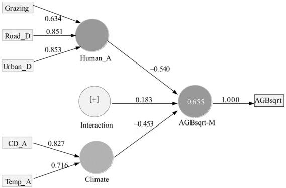
The indicators reflected by either human activities or climate conditions showed positive loadings, ranging from the lowest 0.634 for Grazing to the highest 0.853 for Road_D. The main effects from the human activities and climate factors had negative path coefficients to the endogenous variable (i.e., the modeled AGBsqrt-M) with β = -0.540 and -0.453, respectively. On the contrary, their interaction path coefficient (i.e., Interaction) showed a positive value (β =0.183). This statistic showed that the vegetation was adapting to the human and climate stresses although either higher human activities (Human_A) or climate factors (Climate) alone could result in poor AGB. The interaction term confirmed the complex relationships between the response of AGB and the adaptation of vegetation to human pressure or/and climate pressure. The overall coefficient of determination (R2) for the model reached 0.655, explaining 65.5% of the variance in AGBsqrt from the combination of the main, and interaction of human-climate factors.
Fig. 3 PLS-SEM results with loadings and path coefficients. AGBsqrt-M means the modeled endogenous variable for AGBsqrt and the symbol [+] represents the pairwise product term between the 2 indicators of Climate and the 3 indicators of Human_A (Henseler and Chin, 2010).
3.3 Localized impact from the human activities and climate variations
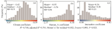
Model estimation began with an examination of the linear relationship between AGB and the human-climate factors. The VIF values (less than 7.5) indicated that the OLS estimates were not biased from global multicollinearity. The condition number reported from GWR (with “ adaptive” Kernel) suggested a lack of local multicollinearity. The OLS and GWR models were further compared by two evaluation parameters (Adjusted R2 and AICc). The comparison indicated that R2 in GWR had been larger than that in OLS (0.681 vs 0.655), and that AICc values in GWR were smaller than that in OLS (590 vs 595), suggesting that the localized impact from the human-climate factors could be identified by GWR modeling. Figure 4 summarizes the distributions (histograms) of the coefficients and the statistical indices of the GWR model between AGBsqrt and the three latent variables (i.e., Climate, Human_A, and Interaction). The distribution histograms of the coefficients indicated that there existed extensive spatial variations in the coefficients estimated at different locations. The coefficient parameter from Human_A had the highest variation (with standard deviation (SD)=0.56) while that from Climate and Interaction varied less (SD=0.15 and 0.21, respectively). From the overall statistical indices in the GWR model, R2 reached 0.718, indicating that the model accounted for 71.8% of the variance for AGBsqrt. Moran’ s I for residual equaled to 0.052 and showed no significance at the 0.05 level (Z-score=0.093 and P=0.925), suggesting that the residuals were spatially random.
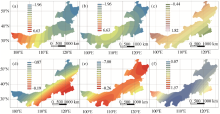
The results in Figure 5 show the contour maps of the factor scores (Figs. 5a-c) and the corresponding regression coefficients by the GWR modeling (Figs. 5d-f). The climate factors (Climate) increased along the direction from the northeast to the southwest, displaying the extremely dry condition combined with relatively high temperature in the southwestern part of IMAR. The human activities (Human_A) showed higher intensities in the middle part where more cities and more populations were located and decreased both eastward and westward. The interaction score decreased along the gradient from the northwest to the southeast. The main effects from the human-climate factors and their interaction effect driving grassland degradation varied greatly across the study area as evidenced from the spatial distributions of GWR coefficients. In the western and northeastern parts, grassland productivity had the most sensitive and negative response to Climate; the southeastern part of the study area observed less sensitive response to Climate. The most sensitive region of vegetation productivity to Human_A was in the western and southeastern areas (with most negative coefficient value) while the least sensitive area was located in the northeast where both Human_A and Climate had relatively low values. Moreover, the interaction coefficient showed spatial variation with the most prominent interaction effect observed in the western and southeastern parts where relatively fewer human settlements were found. This finding may suggest that the vegetation might have adapted to human and climate conditions to some extent (see Section 4.2 for detailed discussion).
Fig. 5 Distributions of interpolated factor scores and the corresponding coefficients from GWR. Input factor scores: (a) Climate; (b) Human_A; (c) Interaction. Output coefficient: (d) Climate coefficient; (e) Human_A coefficient; (f) Interaction coefficient.
4 Discussion
4.1 PLS-SEM applications in socio-ecological systems
A basic framework for applying PLS-SEM model in assessing the cause-effect relationships between the human-climate factors and the grassland productivity was presented. PLS-SEM combines features of multivariate statistical methods such as principal component analysis with multiple regression using iterative regression processes and bootstrapping to maximize the explained variance of the endogenous latent factors. It is thus able to overcome limitations of the first generation analysis tools (Haenlein and Kaplan, 2004; Abdi, 2010). When building such models, the general steps involve conceptualization of potential contribution factors (latent variables), creation and testing of the measurement model (the selection of indicators and the calculation of indicators’ loadings), and fitting and testing of the structure model (path coefficients between the exogenous and endogenous variables). Depending on actual scenarios, the selected factors and the structure of the models could be different. Assisted by the available software package such as SmartPLS, those steps can be readily achieved.
Methodologically, this study has demonstrated the usefulness of using PLS-SEM model to analyze the cause-effect relationship for the grassland ecosystem. At least two advantages were verified in this study. First, PLS-SEM model is useful for analyzing non-normal, multidimensional, and multi-collinear dataset (Henseler et al., 2016; Sarstedt et al., 2016). When a dataset with variables shows high skewness and kurtosis (e.g., the road density in Table 1), PLS-SEM is a more appropriate tool than CB-SEM to test the hypothesis for the multivariate relationships (Hair et al., 2014). Normalization of input indicators is unnecessary as shown by prior researches (e.g., Cassel et al., 1999; Reinartz et al., 2009). However, normalized input could increase the explanation power of the established models and thus researchers should nevertheless consider data distribution since highly skewed data inflate errors and reduce statistical power (Chernick, 2008). In the current study, we used AGBsqrt to get better explanation for its variance from the human-climate factors and their interaction. Second, PLS-SEM allows for a flexible handling of more advanced model elements such as moderator variables or hierarchical component models (Henseler and Chin, 2010; Becker et al., 2012), and it is thus useful to study the interaction effect between multiple factors. The influence of the human-climate factors on AGB was revealed from both the main effects and the interaction effect.
Particular attention should be paid to modeling the interaction effect of multiple factors in PLS-SEM. Henseler and Chin (2010) summarized the four common ways, including the product indicator approach (PIA), 2-stage approach, hybrid approach, and orthogonalizing approach, and they also compared their pros and cons. The PIA, which was first introduced by Busemeyer and Jones (1983) and Kenny and Judd (1984), was adopted in this study through building the product terms with the indicators of the latent independent variable (Climate) and the latent moderator variable (Human_A). Compared to other methods, the PIA and the orthogonalizing approach can provide more accurate predictions (Henseler and Chin, 2010). However, readers should refer to the advantages and limitations of each approach and select the suitable one to better reveal the interaction effect under different contexts. Furthermore, the sample size is also a critical factor. It was recommended that if the sample size is medium to large (which is the case in the current study), PIA should be used (Henseler and Chin, 2010).
4.2 Impact of human-climate factors on vegetation productivity
Previous studies have confirmed that grassland vegetation productivity could be modified by climate variations and human activities (Li et al., 2013; Gang et al., 2014). The relationship between vegetation productivity and the influencing factors may be complex and nonlinear (Tanţ ă u et al., 2014; Liu et al., 2015). Some studies have been conducted to investigate the impacts of climate variations or human activities on vegetation productivity (Wang et al., 2012; Li et al., 2013), but the quantitative assessment of the interaction effect (between human activities and climate factors) is not yet convincingly reported. PLS-SEM provides a promising tool to evaluate both the main effects (from human and climate stresses) and the interaction effect (between human activities and climate factors) on grassland productivity. In the case study, the indicators selected for human activities included the grazing intensity, urbanization intensity and road network intensity while the annually average temperature and climate dryness were selected for the climate factors. The model testing statistics showed that all the indicators were reliable and valid and that the path coefficients were significant. The main effects contributed significantly but negatively to AGBsqrt, suggesting that intensive grazing, dense road network and urban development, or/and high temperature and dry climate in arid regions could lead to poor vegetation productivity, being consistent with the previous studies (Li et al., 2013). More importantly, the interaction effect imposed a significant and positive effect on AGB, revealing that the impact from the climate factors could be mediated by the human activities or vice versa. There are a few possible explanations for such an interaction phenomenon, though further investigation may be required to confirm the explanations. First, the negative effect on vegetation growth could be partially moderated due to vegetation adaptation to intensified human and climate stresses, as vegetation adaptation to human and natural causes has long been reported (Ringrose et al., 2002). Second, recent vegetation restoration programs, e.g., the fragile area protection (protecting vegetation by fencing) introduced mostly in vegetation degraded regions (co-located with intensive human activities) by the Chinese government helped vegetation recovery (Mu et al., 2013). Third, vegetation protection is an important way for human adaptation to climate conditions (O’ Brien et al., 2004) and might have also help to alleviate the negative impact on AGB from high human and climate pressure.
Although PLS-SEM modeling results show that the main effects (from human and climate stresses) imposed a negative impact on grassland productivity whereas the interaction effect (between human activities and climate factors) showed a positive effect, the heterogeneous spatial distribution of the regression coefficients by the GWR modeling suggested that the sensitivity of AGB response to those factors was location-specific. With the recent development of the economy, urban expansion, transportation development, and grazing might have resulted in a significant impact on grassland vegetation (Li et al., 2016). This significant impact was reflected by the factor score of human activities that was higher in the middle part where most key cities (including the capital city Hohhot) were located. Furthermore, the spatial distribution of the GWR coefficients suggest that human activities had substantial but local impact on vegetation productivity, as the coefficient of Human_A showed highest deviation (Figs. 4b and 5e). For example, in the western IMAR, the vegetation showed the most fragile (highest regression coefficient) in response to the pressure from the human activities. Conversely, the climate factors modulated the vegetation productivity at a more uniform or global scale, as indicated by the lower variation of the regression coefficient (Figs. 4a and 5d). It deserves to point out that, from the comparison of the distribution of the climate factors and human activities (Figs. 5a and b), it is likely that humans intended to reduce their activities in the climatically stressed areas. That is, human may adjust its behaviors under unfavorable climate and this adjustment is known as human adaptation (Palmer and Smith, 2014). The GWR modeling also unveiled a spatially varying interaction effect between the human activities and climate factors.
5 Conclusions
This work demonstrated the usefulness of applying PLS-SEM and GWR to evaluating the impact of the human-climate factors on the grassland vegetation productivity in IMAR. The combination of the PLS-SEM and GWR modeling allowed us to explore both the main and interaction effects from the human-climate factors and to understand the spatial variance in the sensitivity of the AGB response to those factors. On-site field data along with other ancillary dataset collected for the typical grassland provided an excellent case study. The framework for developing, testing and evaluating the PLS-SEM model for IMAR was presented. Though only limited variables were taken in the case study, the results from the PLS-SEM did indicate that intensive human activities (including intense grazing, dense road network, and vicinity to urbanized areas) or/and unfavorable climate conditions (i.e., high annual temperature and less water availability) were contributing factors to low AGB. More importantly, the result revealed that the impact on vegetation productivity could be partially alleviated through the interaction effect (between the human activities and climate factors). In addition, the spatially varied sensitivity of the AGB response to the human-climate factors identified by the GWR modeling provided further evidence of the complicated cause-effective relationships existing in the ecosystem. Those findings can serve as critical reference for grassland practitioners to make informed decisions on grassland management.
Acknowledgements
This study was supported by the National Natural Science Foundation of China (41371371) and the Strategic Priority Research Program of the Chinese Academy of Sciences (XDA05050402). We also thank the anonymous reviewers and editors for their constructive comments and suggestions.
The authors have declared that no competing interests exist.
Antle JM, Capalbo SM, Elliott ET, et al. 2001. Research needs for understand ing and predicting the behavior of managed ecosystems: Lessons from the study of agroecosystems. Ecosystems, 4(8): 723-735. [Cited Within:1]
3
Astrachan CB, Patel VK, WanzenriedG. 2014. A comparative study of CB-SEM and PLS-SEM for theory development in family firm research. Journal of Family Business Strategy, 5(1): 116-128. [Cited Within:3]
Bagozzi RP, YiY. 2012. Specification, evaluation, and interpretation of structural equation models. Journal of the Academy of Marketing Science, 40(1): 8-34. [Cited Within:1]
6
BanerjeeU, HineJ. 2016. Interpreting the influence of urban form on household car travel using partial least squares structural equation modelling: some evidence from Northern Ireland . Transportation Planning and Technology, 39(1): 24-44. [Cited Within:1]
7
Becker JM, KleinK, WetzelsM. 2012. Hierarchical latent variable models in PLS-SEM: guidelines for using reflective-formative type models. Long Range Planning, 45(5-6): 359-394. [Cited Within:1]
8
Bollen KA. 1989. Structural Equations with Latent Variables. New York: Wiley, 10-17. [Cited Within:1]
Busemeyer JR, Jones LE. 1983. Analysis of multiplicative combination rules when the causal variables are measured with error. Psychological Bulletin, 93(3): 549-562. [Cited Within:1]
11
CasselC, HacklP, Westlund AH. 1999. Robustness of partial least-squares method for estimating latent variable quality structures. Journal of Applied Statistics, 26(4): 435-446. [Cited Within:1]
12
Chapin FS, Sala OE, Huber-SannwaldE. 2001. Global Biodiversity in a Changing Environment: Scenarios for the 21st Century. New York: Springer, 121-137. [Cited Within:1]
13
Chernick MR. 2008. Bootstrap Methods: A Guide for Practitioners and Researchers (2nd ed. ). Hoboken: Wiley, 78-96. [Cited Within:1]
14
Chin WW. 1998. Commentary: Issues and opinion on structural equation modeling. MIS Quarterly, 22(1): 7-16. [Cited Within:6]
15
Chin WW, Marcolin BL, Newsted PR. 2003. A partial least squares latent variable modeling approach for measuring interaction effects: Results from a Monte Carlo simulation study and an electronic-mail emotion/adoption study. Information Systems Research, 14(2): 189-217. [Cited Within:1]
16
Chin WW. 2010How to write up and report PLS analyses. In: Vinzi V E, Chin W W, Henseler J, et al. Hand book of Partial Least Squares: Concepts, Methods and Applications. Berlin Heidelberg: Springer, 655-690. [Cited Within:1]
17
ChristensenL, Coughenour MB, Ellis JE, et al. 2004. Vulnerability of the Asian typical steppe to grazing and climate change. Climatic Change, 63(3): 351-368. [Cited Within:1]
18
Cutler NA, Belyea LR, Dugmore AJ. 2008. The spatiotemporal dynamics of a primary succession. Journal of Ecology, 96(2): 231-246. [Cited Within:1]
19
De LuisM, RaventósJ, González-Hidalgo JC. 2006. Post-fire vegetation succession in Mediterranean gorse shrubland s. Acta Oecologica, 30(1): 54-61. [Cited Within:1]
20
EisenhauerN, Bowker MA, Grace JB, et al. 2015. From patterns to causal understand ing: Structural equation modeling (SEM) in soil ecology. Pedobiologia, 58(2-3): 65-72. [Cited Within:1]
21
FanY, Chen JQ, ShirkeyG, et al. 2016. Applications of structural equation modeling (SEM) in ecological studies: an updated review. Ecological Processes, 5: 19. [Cited Within:1]
22
FilatovaT, Verburg PH, Parker DC, et al. 2013. Spatial agent-based models for socio-ecological systems: Challenges and prospects. Environmental Modelling & Software, 45: 1-7. [Cited Within:1]
23
FornellC, Larcker DF. 1981. Evaluating structural equation models with unobservable variables and measurement error. Journal of Marketing Research, 18(1): 39-50. [Cited Within:1]
24
Gang CC, ZhouW, Chen YZ, et al. 2014. Quantitative assessment of the contributions of climate change and human activities on global grassland degradation. Environmental Earth Sciences, 72(11): 4273-4282. [Cited Within:3]
25
GefenD, StraubD, Boudreau MC. 2000. Structural equation modeling and regression: Guidelines for research practice. Communications of the Association for Information Systems, 4(1): 7. [Cited Within:2]
26
GeisserS. 1974. A predictive approach to the rand om effect model. Biometrika, 61(1): 101-107. [Cited Within:1]
27
HaenleinM, Kaplan AM. 2004. A Beginner’s guide to partial least squares analysis. Understand ing Statistics, 3(4): 283-297. [Cited Within:2]
28
Hair Jr JF, Black WC, Babin BJ, et al. 2009. Multivariate Data Analysis: A Global Perspective (7th ed. ). New Jersey: Prentice Hall, Inc. , 730-738. [Cited Within:2]
Hair Jr JF, SarstedtM, Ringle CM, et al. 2012. An assessment of the use of partial least squares structural equation modeling in marketing research. Journal of the Academy of Marketing Science, 40(3): 414-433. [Cited Within:2]
31
Hair Jr JF, Hult G TM, Ringle CM, et al. 2014. A Primer on Partial Least Squares Structural Equation Modeling (PLS-SEM). California: SAGE Publication, Inc. , 1-23. [Cited Within:5]
32
HenselerJ, Ringle CM, Sinkovics RR. 2009. The use of partial least squares path modeling in international marketing, Volume 20). In: Sinkovics R R, Ghauri P N. New Challenges to International Marketing (Advances in International Marketing. Bingley: Emerald Group Publishing Limited, 277-319. [Cited Within:1]
33
HenselerJ, Chin WW. 2010. A comparison of approaches for the analysis of interaction effects between latent variables using partial least squares path modeling. Structural Equation Modeling: A Multidisciplinary Journal, 17(1): 82-109. [Cited Within:4]
34
HenselerJ, SarstedtM. 2013. Goodness-of-fit indices for partial least squares path modeling. Computational Statistics, 28(2): 565-580. [Cited Within:1]
35
HenselerJ, HubonaG, Ray PA. 2016. Using PLS path modeling in new technology research: updated guidelines. Industrial Management & Data Systems, 116(1): 2-20. [Cited Within:2]
36
Hulland J. 1999. Use of partial least squares (PLS) in strategic management research: a review of four recent studies. Strategic Management Journal, 20(2): 195-204. [Cited Within:5]
37
Hutchinson MF. 1999. ANUSPLIN Version 4. 0 User Guide. Canberra: The Australian National University. [Cited Within:1]
38
Jöreskog KG. 1971. Statistical analysis of sets of congeneric tests. Psychometrika, 36(2): 109-133. [Cited Within:1]
39
Jöreskog KG, Wold H O A. 1982. The ML and PLS techniques for modeling with latent variables: Historical and comparative aspects. In: Jöreskog K G, Wold H O A. Systems under Indirect Observation: Part I. Amsterdam: North-Holland , 263-270. [Cited Within:1]
40
Jöreskog KG. 1993. Testing structural equation models. In: Bollen K A, Long J S. Testing Structural Equation Models. California: Sage Publication, Inc. , 294-316. [Cited Within:1]
41
Kenny DA, Judd CM. 1984. Estimating the nonlinear and interactive effects of latent variables. Psychological Bulletin, 96(1): 201-210. [Cited Within:1]
42
Lauenroth WK, Burke IC, Gutmann MP. 1999. The structure and function of ecosystems in the Central North American grassland region. Great Plains Research, 9(2): 223-259. [Cited Within:1]
43
LiS, Xie YC, Brown DG, et al. 2013. Spatial variability of the adaptation of grassland vegetation to climatic change in Inner Mongolia of China. Applied Geography, 43: 1-12. [Cited Within:4]
44
Li XB, Li RH, Li GQ, et al. 2016. Human-induced vegetation degradation and response of soil nitrogen storage in typical steppes in Inner Mongolia, China. Journal of Arid Environments, 124: 80-90. [Cited Within:1]
45
Li XX, Wang LX, ZhangJ, et al. 2014. Exploration of ecological factors related to the spatial heterogeneity of tuberculosis prevalence in P. R. China. Global Health Action, 7, doi: DOI:10.3402/gha.v7.23620. [Cited Within:1]
46
LiuM, Liu GH, GongL, et al. 2014. Relationships of biomass with environmental factors in the grassland area of Hulunbuir, China. PLoS ONE, 9(7): e102344, doi: DOI:10.1371/journal.pone.0102344. [Cited Within:1]
47
Liu YX, Liu XF, Hu YN, et al. 2015. Analyzing nonlinear variations in terrestrial vegetation in China during 1982-2012. Environmental Monitoring and Assessment, 187(11): 722. [Cited Within:1]
48
Lowry PB, GaskinJ. 2014. Partial least squares (PLS) structural equation modeling (SEM) for building and testing behavioral causal theory: when to choose it and how to use it. IEEE Transactions on Professional Communication, 57(2): 123-146. [Cited Within:1]
49
MoneckeA, LeischF. 2012. semPLS: structural equation modeling using partial least squares. Journal of Statistical Software, 48(3): 23662. [Cited Within:2]
50
Moore C WE. 1966. Distribution of grassland s. In: Barnard C. Grasses and Grassland s. New York: Macmillan, 182-205. [Cited Within:1]
51
Mu SJ, Chen YZ, Li JL, et al. 2013. Grassland dynamics in response to climate change and human activities in Inner Mongolia, China between 1985 and 2009. The Rangeland Journal, 35(3): 315-329. [Cited Within:2]
52
O’BrienK, LeichenkoR, KelkarU, et al. 2004. Mapping vulnerability to multiple stressors: climate change and globalization in India. Global Environmental Change, 14(4): 303-313. [Cited Within:1]
53
Palmer PI, Smith MJ. 2014. Earth systems: Model human adaptation to climate change. Nature, 512(7515): 365-366. [Cited Within:1]
Reinartz WJ, HaenleinM, HenselerJ. 2009. An empirical comparison of the efficacy of covariance-based and variance-based SEM. International Journal of Research in Marketing, 26(4): 332-344. [Cited Within:1]
56
RingroseS, Chipanshi AC, MathesonW, et al. 2002. Climate- and human-induced woody vegetation changes in Botswana and their implications for human adaptation. Environmental Management, 30(1): 98-109. [Cited Within:1]
57
SarstedtM, Ringle CM, SmithD, et al. 2014. Partial least squares structural equation modeling (PLS-SEM): A useful tool for family business researchers. Journal of Family Business Strategy, 5(1): 105-115. [Cited Within:2]
58
SarstedtM, Hair JF, Ringle CM, et al. 2016. Estimation issues with PLS and CBSEM: Where the bias lies!Journal of Business Research, 69(10): 3998-4010. [Cited Within:1]
59
Sha ZY, Zhong JL, Bai YF, et al. 2016. Spatio-temporal patterns of satellite-derived grassland vegetation phenology from 1998 to 2012 in Inner Mongolia, China. Journal of Arid Land , 8(3): 462-477. [Cited Within:1]
60
Shen WW, Xiao WZ, WangX. 2016. Passenger satisfaction evaluation model for urban rail transit: A structural equation modeling based on partial least squares. Transport Policy, 46: 20-31. [Cited Within:1]
61
Stannard CA, Aspinall RJ. 2011. Meeting the challenges of modelling coupled human-environmental systems-GLP Nodal Office of Integration and Modelling. Procedia Environmental Sciences, 6: 194-198. [Cited Within:1]
62
StoneM. 1974. Cross-validatory choice and assessment of statistical predictions. Journal of the Royal Statistical Society: Series B (Methodological), 36(2): 111-147. [Cited Within:1]
63
Sun YL, Yang YL, ZhangL, et al. 2015. The relative roles of climate variations and human activities in vegetation change in North China. Physics and Chemistry of the Earth, Parts A/B/C, 87-88: 67-78. [Cited Within:1]
64
Surridge B WJ, BizziS, CastellettiA. 2014. A framework for coupling explanation and prediction in hydroecological modelling. Environmental Modelling & Software, 61: 274-286. [Cited Within:2]
65
TanţăuI, FeurdeanA, De Beaulieu JL, et al. 2014. Vegetation sensitivity to climate changes and human impact in the Harghita Mountains (Eastern Romanian Carpathians) over the past 15, 000 years. Journal of Quaternary Science, 29(2): 141-152. [Cited Within:1]
66
TenenhausM, Vinzi VE, Chatelin YM, et al. 2005. PLS path modeling. Computational Statistics & Data Analysis, 48(1): 159-205. [Cited Within:2]
67
WabiriN, ShisanaO, ZumaK, et al. 2016. Assessing the spatial nonstationarity in relationship between local patterns of HIV infections and the covariates in South Africa: A geographically weighted regression analysis. Spatial and Spatio-temporalEpidemiology, 16: 88-99. [Cited Within:1]
68
WangT, Sun JG, HanH, et al. 2012. The relative role of climate change and human activities in the desertification process in Yulin region of northwest China. Environmental Monitoring and Assessment, 184(12): 7165-7173. [Cited Within:1]
69
Wold H OA. 1982. Soft modeling: The basic design and some extensions. In: Jöreskog K G, Wold H O A. Systems under Indirect Observations: Part II. Amsterdam: North-Holland , 1-54. [Cited Within:2]
70
Wold H OA. 1985. Partial least squares. In: Kotz S, Johnson N L. Encyclopedia of Statistical Sciences. New York: Wiley, 581-591. [Cited Within:1]
71
Zhang JH, Huang YM, Chen HY, et al. 2016. Effects of grassland management on the community structure, aboveground biomass and stability of a temperate steppe in Inner Mongolia, China. Journal of Arid Land , 8(3): 422-433. [Cited Within:1]
72
Zhang YJ, Li XM, Wang AM, et al. 2015. Density and diversity of OpenStreetMap road networks in China. Journal of Urban Management, 4(2): 135-146. [Cited Within:1]
1
2010
0.0
0.0
... Abdi, 2010) ...
1
2001
0.0
0.0
... There are three levels of models in studying SES, namely, loose coupling, tight coupling, and integrated modeling (Antle et al ...
3
2014
0.0
0.0
... Over the last decade, structural equation modeling (SEM) has been applied in many scientific disciplines (Astrachan et al ...
... While CB-SEM estimates model parameters so that the discrepancy between the estimated and the sample covariance matrices is minimized, PLS-SEM maximizes the explained variance of the endogenous latent variables by estimating partial model relationships in an iterative sequence of ordinary least squares (OLS) regressions (Astrachan et al ...
... Astrachan et al ...
1
1988
0.0
0.0
1
2012
0.0
0.0
... It is capable of fully revealing the inner characteristics of the observed data (Bagozzi and Yi, 2012) ...
1
2016
0.0
0.0
... Banerjee and Hine, 2016) ...
1
2012
0.0
0.0
... Becker et al ...
1
1989
0.0
0.0
... Overall, SEM model provides an effective tool to assess latent variables at the measurement model and test the relationships between the latent variables on the structural model (Bollen, 1989 ...
2
1998
0.0
0.0
... GWR modeling is an exploratory technique mainly intended to identify where non-stationary takes place on the map, namely exploring spatial heterogeneity (Brunsdon et al ...
... The spatial distribution of the regression coefficients could indicate how sensitively the AGB responded to any change in the corresponding variables (Brunsdon et al ...
1
1983
0.0
0.0
1
1999
0.0
0.0
... , Cassel et al ...
1
2001
0.0
0.0
... Chapin et al ...
1
2008
0.0
0.0
... However, normalized input could increase the explanation power of the established models and thus researchers should nevertheless consider data distribution since highly skewed data inflate errors and reduce statistical power (Chernick, 2008) ...
6
1998
0.0
0.0
... SEM possesses substantial advantages over the first generation techniques (Chin, 1998 ...
... In this PLS-SEM model specification, the reflective type was specified because the constructs were reflectively measured latent variables that did not share a common cause but rather formed a general concept that mediated the influence on subsequent endogenous variables (Chin, 1998) ...
... ) were also examined because they indicated the strengths of relationships between the exogenous and the endogenous variables (Chin, 1998) ...
... 7 is used as a benchmark for modest CR (Chin, 1998 ...
... For valid discriminant of construct, AVE shared on itself should be higher than that with other constructs (Chin, 1998) ...
... values indicate the strengths of relationships between constructs (Chin, 1998) ...
1
2003
0.0
0.0
... For instance, the product indicator approach (PIA) has been developed to quantitatively reflect the magnitude of such a coupled effect (Chin et al ...
1
0.0
0.0
... , Chin, 2010 ...
1
2004
0.0
0.0
... Specifically, the increasing human population and intensified grazing coupled with arid climate condition were identified as the primary threats to the sustainable development of the grassland ecology (Christensen et al ...
1
2008
0.0
0.0
... Cutler et al ...
1
2006
0.0
0.0
... Understanding the factors affecting grassland productivity is increasingly critical to the conservation and, in some cases, to the restoration of these fragile ecosystems (De Luis et al ...
1
2015
0.0
0.0
... HSEM, also known as multilevel SEM, analyzes hierarchically clustered data by specifying the direct and indirect causal effect between clusters (Eisenhauer et al ...
1
2016
0.0
0.0
... Fan et al ...
1
2013
0.0
0.0
... Filatova et al ...
1
1981
0.0
0.0
... It is tested through analysis of average variance extracted by using the criteria that a construct should share more variance with its measures than that with other constructs in the model (Fornell and Larcker, 1981) ...
3
2014
0.0
0.0
... Gang et al ...
... Climate change and human interference are commonly recognized as the two broad underlying drivers that lead to grassland degradation (Gang et al ...
... Gang et al ...
2
2000
0.0
0.0
... Gefen et al ...
... Convergent validity of the construct is determined by average variance extracted (AVE) (Gefen et al ...
1
1974
0.0
0.0
... value could also be calculated as a criterion of predictive relevance (Geisser, 1974 ...
2
2004
0.0
0.0
... In the measurement model (or outer model), a set of latent variables are aggregated from the observable data to form an underlying concept, which greatly reduces the dimensionality of the original variables and makes the data easier to understand (Haenlein and Kaplan, 2004 ...
... It is thus able to overcome limitations of the first generation analysis tools (Haenlein and Kaplan, 2004 ...
2
2009
0.0
0.0
... SEM has been popular in many disciplines and allows great flexibility on equation specification (Hair et al ...
... PLS-SEM assumes a minimum of data requirement and is an excellent tool for studying the causal relationships between multiple variables in ecological systems (Hair et al ...
4
2011
0.0
0.0
... Hair et al ...
... Lastly, the significance of the outer model loadings for the indicators and the inner path coefficients indicating the relationship between the latent variables were tested by using the bootstrapping function (Hair et al ...
... Hair et al ...
... 5 is usually viewed as acceptable (Hair et al ...
2
2012
0.0
0.0
... Hair et al ...
... PLS-SEM is essentially a regression-based modeling approach, which uses a component-based technique in analyzing path models (Hair et al ...
5
2014
0.0
0.0
... Hair et al ...
... Second, PLS-SEM has the advantage of the flexibility for the use of a single measurement construct (Hair et al ...
... Therefore, potential collinearity between predictor constructs in the structural model should be tested (Hair et al ...
... 25 (Hair et al ...
... , the road density in Table 1), PLS-SEM is a more appropriate tool than CB-SEM to test the hypothesis for the multivariate relationships (Hair et al ...
1
0.0
0.0
... In recent years, PLS-SEM has expanded rapidly with recognition of being a distinctive and innovative multivariate analysis method (Henseler et al ...
4
2010
0.0
0.0
... A few approaches have been proposed to analyze the interaction effect between multiple latent variables for PLS-SEM (Henseler and Chin, 2010) ...
... Second, PLS-SEM allows for a flexible handling of more advanced model elements such as moderator variables or hierarchical component models (Henseler and Chin, 2010 ...
... Compared to other methods, the PIA and the orthogonalizing approach can provide more accurate predictions (Henseler and Chin, 2010) ...
... It was recommended that if the sample size is medium to large (which is the case in the current study), PIA should be used (Henseler and Chin, 2010) ...
1
2013
0.0
0.0
... PLS-SEM does not have a standard goodness-of-fitting statistic (Henseler and Sarstedt, 2013) ...
2
2016
0.0
0.0
... Henseler et al ...
... First, PLS-SEM model is useful for analyzing non-normal, multidimensional, and multi-collinear dataset (Henseler et al ...
5
1999
0.0
0.0
... In the first stage, the reliability and validity tests were performed for the outer model (Hulland, 1999 ...
... 4, in a reflective model, to show that the construct is able to explain the indicator (Hulland, 1999) ...
... It is estimated to ensure that the items assumed to measure the construct are correct while do not actually measure other constructs (Hulland, 1999) ...
... Discriminant validity indicates the extent to which a given construct is different from other constructs (Hulland, 1999) ...
... Instead, the structural model evaluation is carried out to assess the relationship between constructs and endogenous latent variables in respect of variance accounted (Hulland, 1999) ...
1
1999
0.0
0.0
... 1 km using an ANUSPLIN approach (Hutchinsom, 1999) ...
1
1971
0.0
0.0
... s composite (construct) reliability (CR) (J#cod#x000f6 ...
1
0.0
0.0
... , the covariance-based technique or CB-SEM (J#cod#x000f6 ...
1
0.0
0.0
1
1984
0.0
0.0
1
1999
0.0
0.0
... Grasslands are sensitive to human activities and weather variations (Lauenroth et al ...
4
2013
0.0
0.0
... , Li et al ...
... 2 Impact of human-climate factors on vegetation productivityPrevious studies have confirmed that grassland vegetation productivity could be modified by climate variations and human activities (Li et al ...
... Li et al ...
... The main effects contributed significantly but negatively to AGBsqrt, suggesting that intensive grazing, dense road network and urban development, or/and high temperature and dry climate in arid regions could lead to poor vegetation productivity, being consistent with the previous studies (Li et al ...
1
2016
0.0
0.0
... With the recent development of the economy, urban expansion, transportation development, and grazing might have resulted in a significant impact on grassland vegetation (Li et al ...
1
2014
0.0
0.0
... Li et al ...
1
2014
0.0
0.0
... As a second-generation multivariate statistical approach, SEM has played a prominent role in the SES (Liu et al ...
1
2015
0.0
0.0
... Liu et al ...
1
2014
0.0
0.0
... Lowry and Gaskin, 2014) ...
2
2012
0.0
0.0
... In the structural model (or inner model), the latent variables are connected with each other according to a substantive theory in the form of simple connected digraphs (Monecke and Leisch, 2012) ...
... Monecke and Leisch, 2012) ...
1
0.0
0.0
... 1 IntroductionNatural grasslands and savannas occupy nearly half of the terrestrial area of the globe (Moore, 1966 ...
2
2013
0.0
0.0
... Previous studies revealed that grassland productivity was affected by human activities and climate fluctuations (Mu et al ...
... , the fragile area protection (protecting vegetation by fencing) introduced mostly in vegetation degraded regions (co-located with intensive human activities) by the Chinese government helped vegetation recovery (Mu et al ...
1
2004
0.0
0.0
... Third, vegetation protection is an important way for human adaptation to climate conditions (O#cod#x02019 ...
1
2014
0.0
0.0
... That is, human may adjust its behaviors under unfavorable climate and this adjustment is known as human adaptation (Palmer and Smith, 2014) ...
1
2016
0.0
0.0
... Polhill et al ...
1
2009
0.0
0.0
... Reinartz et al ...
1
2002
0.0
0.0
... First, the negative effect on vegetation growth could be partially moderated due to vegetation adaptation to intensified human and climate stresses, as vegetation adaptation to human and natural causes has long been reported (Ringrose et al ...
2
2014
0.0
0.0
... Sarstedt et al ...
... Designed for working with multiple equations simultaneously, SEM offers a number of advantages over the traditional statistics such as regression analysis or factor analysis (Sarstedt et al ...
1
2016
0.0
0.0
... Sarstedt et al ...
1
2016
0.0
0.0
... 200 mm), the middle and the east is a semi-arid region (annual precipitation in the ranges of 200-400 and 400-600 mm, respectively) (Sha et al ...
1
2016
0.0
0.0
... First, unlike CB-SEM that requires the multivariate normal distribution for the input data, PLS-SEM relaxes the assumption of normal distribution and can obtain explicitly the estimated latent variable scores in the process of parameter estimation (Shen et al ...
1
2011
0.0
0.0
... While much attention has been paid to studying systemic changes of ecological and economic systems independently, the attempt for taking a coupled SES approach is still rare (Stannard and Aspinall, 2011 ...
1
1974
0.0
0.0
... Stone, 1974) ...
1
2015
0.0
0.0
... Sun et al ...
2
2014
0.0
0.0
... Surridge et al ...
... Third, PLS-SEM is suitable for predictive research, which is usually not the case for CB-SEM (Surridge et al ...
1
2014
0.0
0.0
... The relationship between vegetation productivity and the influencing factors may be complex and nonlinear (Tan#cod#x00163 ...
2
2005
0.0
0.0
... PLS-SEM is a soft-modeling-technique with minimum demands regarding the measurement scales, sample sizes, and residual distributions (Tenenhaus et al ...
... Therefore, they were treated as error free substitutes for the indicators (Tenenhaus et al ...
1
2016
0.0
0.0
... Multicollinearity between input variables was proved to be a problem in regression analysis and needs to be checked through variance inflation factor (VIF) and condition number, where VIF values greater than 10 indicated presence of multicollinearity (Wabiri et al ...
1
2012
0.0
0.0
... Some studies have been conducted to investigate the impacts of climate variations or human activities on vegetation productivity (Wang et al ...
2
0.0
0.0
... reskog, 1993) and the variance-based partial least square or PLS-SEM (Wold, 1982, 1985) ...
... reskog and Wold, 1982), earlier studies have focused primarily on CB-SEM ...
1
0.0
0.0
... reskog, 1993) and the variance-based partial least square or PLS-SEM (Wold, 1982, 1985) ...
1
2016
0.0
0.0
... Zhang et al ...
1
2015
0.0
0.0
... Two vector layers about the road network and urbanized areas (including cities and villages) were extracted from the publicly available OpenStreetMap dataset (Zhang et al ...
Assessing the impacts of human activities and climate variations on grassland productivity by partial least squares structural equation modeling (PLS-SEM)
[SHA Zongyao1,*, XIE Yichun2, TAN Xicheng1, BAI Yongfei3, LI Jonathan4, LIU Xuefeng5]


 , XIE Yichun